GRPO on flow matching models
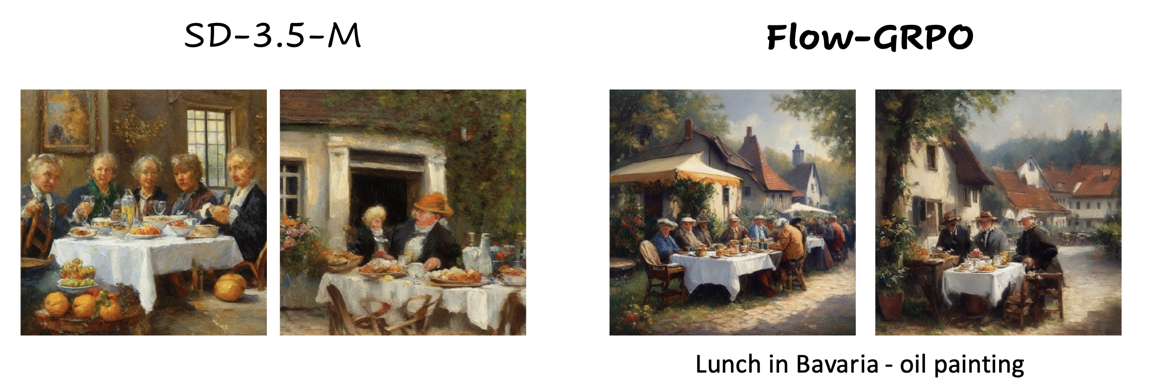
How RL post-training can influence the visual quality of images generated by flow-based models.
Images from Flow-GRPO: Training Flow Matching Models via Online RL (Jie Liu et al., 2025). Cropped; captions reformatted.
RL post-training of language models and agents has become extremely popular recently and has boosted model performance across a wide range of tasks like reasoning and coding. Naturally, if you're working with flow matching based models, you're probably wondering how you can apply these techniques to your model and whether or not it's worth it.
I'm curious about this myself so this is a place where I document my learning about the topic. Of course, you can go and read the paper and implementations yourself.
Flow matching
A short overview again on flow matching, we'll stick with this notation throughout the blog post. The core idea of flow matching is to learn a transform from noise to the clean data distribution. With sufficient training this can function as a generative model at inference, producing anything from images, AI-slop videos to robot actions. Stepping from one noisy latent to the next less noisy latent during flow matching inference is a deterministic process, which will come back to bite us in a few paragraphs.
Sample from the data distribution: \(x_0 \sim X_0\)
Noise sample: \(x_1 \sim X_1\)
Rectified flow: \(x_\tau = (1-\tau)x_0 + \tau x_1\)
Flow matching timestep: \(\tau \in [0,1]\)
Velocity field (the vector pointing from data distribution sample to noise sample): \(v = x_1 - x_0\)
Flow matching objective: \[ \mathcal{L}(\theta) = \mathbb{E}_{\tau, x_0, x_1} \left[ \left\| v - v_\theta(x_\tau,\tau) \right\|_2^2 \right] \]
GRPO
You're probably familiar with the DeepSeekMath paper and how it popularised a way to train reasoning models for math etc. with reinforcement learning on top of LLMs. If you managed to put off reading the paper until now, this is a quick overview. For policy gradient methods in reinforcement learning you usually have an actor and a critic, like for Proximal Policy Optimisation (PPO). However, training the critic requires the additional critic model and its training, which can be prohibitively expensive for large models. Group Relative Policy Optimisation (GRPO) avoids training a critic by sampling some G policy rollouts from the same starting point and computing the relative advantage between them to judge which of these rollouts were better and which ones were worse: \[ \hat{A}^i = \frac{ R^i - \operatorname{mean}(\{R^j\}_{j=1}^{G}) }{ \operatorname{std}(\{R^j\}_{j=1}^{G}) } \]
For G=4 with binary rewards you could have \(R = [1, 0, 1, 1]\), producing normalized advantages \(\hat{A} = [0.577, -1.732, 0.577, 0.577]\).
Policy probability ratio: \[ r_t^i(\theta) = \frac{ \pi_\theta(a_t^i \mid s_t^i) }{ \pi_{\theta_{\mathrm{old}}}(a_t^i \mid s_t^i) } \]
This ratio just tells you how much more or less likely a transition you received from your old policy is under your new policy. Implementing this, you would sample your transitions under the old policy and store something like \((s_t, a_t, \log \pi_{\mathrm{old}}(a_t \mid s_t))\), along with the resulting rewards and advantages. Then, during training, you would evaluate \(\log \pi_\theta(a_t \mid s_t)\) under the current model, which allows you to calculate the ratio \(r_t\).
GRPO objective: \[ \mathcal{J}_{\mathrm{GRPO}}(\theta) = \mathbb{E} \left[ \frac{1}{G} \sum_{i=1}^{G} \frac{1}{T} \sum_{t=0}^{T-1} \left( \min \left( r_t^i(\theta)\hat{A}^i, \operatorname{clip} \left( r_t^i(\theta), 1-\epsilon, 1+\epsilon \right) \hat{A}^i \right) - \beta D_{\mathrm{KL}}(\pi_\theta \| \pi_{\mathrm{ref}}) \right) \right] \]
So the update objective combines the group-relative advantage \(\hat{A}^i\) with the likelihood ratio \(r_t^i(\theta)\), clipped by \(\epsilon\) to prevent excessively large updates, and includes a KL-divergence regularization term. The latter term is supposed to keep you close to your original policy when updating.
How to combine
You can reformulate the flow-matching denoising process as an MDP, where \(t\) indexes the discrete MDP step and \(\tau_t\) is its continuous flow time. The state is \(s_t = (c, \tau_t, x_{\tau_t})\), including the context, flow time, and current point in the denoising process. The action is \(a_t = x_{\tau_{t+1}}\), the next more-denoised point on the trajectory. This makes the stochastic transition distribution parameterized by the flow \(v_\theta\) the policy to optimize. As mentioned above however, the inference sampling process is generally deterministic for flow matching.
To solve this mismatch, the authors in Flow-GRPO (https://arxiv.org/abs/2505.05470) propose substituting the ODE during training rollouts with an SDE. With the correct score and the same initial distribution, this construction exactly preserves the ODE’s marginal probability densities in continuous time: at a fixed noise level, the distribution over particles is the same, while individual trajectories differ due to the injected noise.
The basic Flow-ODE is \[ d x_\tau = v_\tau(x_\tau)\,d\tau \]
with inserted SDE: \[ d x_\tau = \left[ v_\tau(x_\tau) - \frac{g(\tau)^2}{2} \nabla_x \log p_\tau(x_\tau) \right] d\tau + g(\tau)\,dW_\tau \]
Here you first add noise with \(g(\tau)\,dW_\tau\), giving you the desired randomness but spreading probability mass. You compensate for this using the score term, which points toward increasing probability density. Denoising integrates \(\tau: 1 \to 0\), so \(d\tau \lt 0\) and the minus sign puts that step along \(+\nabla_x \log p_\tau\). This fits nicely with flow matching because
\[ \log p_\tau(x_\tau \mid x_0) = \text{const} -\frac{\left\|x_\tau-(1-\tau)x_0\right\|_2^2}{2\tau^2}, \qquad x_\tau \mid x_0 \sim \mathcal{N}\!\left((1-\tau)x_0,\tau^2I\right). \]
Using the interpolation equation gives
\[ \nabla_{x_\tau}\log p_\tau(x_\tau \mid x_0) = -\frac{x_1}{\tau}. \]
The interpolation also gives \(x_1 = x_\tau + (1-\tau)v\). Marginalizing over \(x_0\) gives
\[ \nabla_x\log p_\tau(x) = -\frac{x+(1-\tau)\,\mathbb E[x_1-x_0\mid x_\tau=x]}{\tau}. \]
The learned velocity \(v_\theta(x,\tau)\) approximates this conditional expectation. Substituting it into the score and discretizing with Euler–Maruyama gives
\[ x_{\tau+\Delta \tau} = x_\tau + \left[ v_\theta(x_\tau,\tau) + \frac{g(\tau)^2}{2\tau} \left( x_\tau+(1-\tau)v_\theta(x_\tau,\tau) \right) \right]\Delta \tau + g(\tau)\sqrt{|\Delta \tau|}\epsilon \]
with
\[ \epsilon \sim \mathcal{N}(0,I), \qquad g(\tau) = a\sqrt{\frac{\tau}{1-\tau}} \]
You can find interesting ablations about the hyperparameter \(a\) in the Flow-GRPO paper. Mainly, \(a\) can somewhat drive the exploration process in this formulation since it decides how much noise to add. The Euler–Maruyama transition is Gaussian.
\[ \pi_\theta(x_{\tau+\Delta \tau}\mid x_\tau,c) = \mathcal{N} \left( \mu_\theta, g(\tau)^2|\Delta \tau|I \right), \]
We can calculate the KL divergence term in closed form. The policy and reference model have the same transition variance, so
\[ D_{\mathrm{KL}}(\pi_\theta\|\pi_{\mathrm{ref}}) = \frac{ \left\|\mu_\theta-\mu_{\mathrm{ref}}\right\|_2^2 }{ 2g(\tau)^2|\Delta \tau| }. \] .
There are of course further, interesting ablations in the Flow-GRPO paper that I recommend you checking out. Here we want to focus more on implementation and applications now.
How to implement with Wan2.1
I'm trying to use the same notation as above.
The normal Wan2.1 implementation (https://github.com/Wan-Video/Wan2.1/tree/main) would do something like this:
latent = # x_1

for _, tau in enumerate(timesteps): # timesteps here are the amount of integration steps we do for inference

    v_theta_cond = self.model(latent, tau, context) # v_theta(x_tau, tau, c)
    v_theta_uncond = self.model(latent, tau) # v_theta(x_tau, tau, empty_context)
    v_theta = v_theta_uncond + guide_scale * (v_theta_cond - v_theta_uncond) # CFG-velocity v_theta_CFG

    latent = scheduler.step(v_theta, tau, latent) # x_tau_next
We're looking at a code example from the Flow-GRPO github: https://github.com/yifan123/flow_grpo for SDE injection for WAN2.1. The variable names are changed since I hope that makes it easier to follow the blog post entirely.
class SDEScheduler:
    def step(v_theta, timestep, latent):
        tau = self.sigmas[step_index]  # discussed below
        tau_next = self.sigmas[step_index + 1]

        d_tau = tau_next - tau

        sigma_max = self.sigmas[1]  # discussed below
        sigma_min = self.sigmas[-1]  # 0.0, the scheduler appends a zero terminal sigma

        g_tau = sigma_min + (sigma_max - sigma_min) * tau

        mu_theta = (latent + (v_theta + g_tau**2 / (2 * tau) * (latent + (1 - tau) * v_theta)) * d_tau)

        std_tau = g_tau * torch.sqrt(-d_tau)

        # During rollout we actually sample the next latent
        if latent_next is None:
            epsilon = torch.randn_like(latent)
            latent_next = mu_theta + std_tau * epsilon

        # Evaluate the log_prob under sampled transition
        log_prob = (
            -((latent_next.detach() - mu_theta) ** 2) / (2 * std_tau**2)
            - torch.log(std_tau)
            - 0.5 * math.log(2 * math.pi)
        )

        log_prob = log_prob.mean(dim=tuple(range(1, log_prob.ndim)))

        if old_log_prob is not None:
            policy_ratio = torch.exp(log_prob - old_log_prob)  # During training calculate the ratio
So this is basically the implementation of what we derived above. If you've read closely you'll find two differences:
- g(tau) is just the linear interpolation here instead of the proposed a * sqrt(tau/(1-tau)). So the Wan2.1 Flow-GRPO implementation in the repo differs from the one in the paper. The square-root form is what most of the other implementations in the repo use. MixGRPO (https://github.com/Tencent-Hunyuan/MixGRPO), which is what HunyuanVideo 1.5 (https://arxiv.org/abs/2511.18870) uses for its I2V RLHF, keeps the square-root form with the same \(a = 0.7\) as well.
- The ratio uses the mean over the latent dimension for the log probs, instead of the sum, which would be aligned with what we derived above. This is actually what all other implementations in the repo use as well and someone did ask about this in a github issue (#143), where the author mentions the sum would lead to instability even after adjusting clipping. To me, that would make sense if you have a very high-dimensional latent, you can be a bit more robust against small changes.
Should you apply flow-grpo to your flow matching project?
- Speed: During training, we need the current and next latent for each transition whose log-probability we re-evaluate under the updated policy. Storing these transitions can become expensive, especially for video models, although we only need to retain the transitions we intend to train on. You could inject noise only into some and for the rest use an ODE approach or restrict which transitions to train on (Flow-GRPO-Fast, DanceGRPO are a good starting point for these approaches). Additionally, RL rollouts are of course expensive (especially for video models or similar) and there's always a consideration about learning signal density (https://thinkingmachines.ai/blog/lora).
- Inference Sampler: Wan2.1 uses multi-step solvers like the FlowUniPCMultistepScheduler at inference time, which increases inference speed and quality but is not directly compatible with what we derived above. These multistep solvers use information from previous model evaluations to provide a higher-order update to the denoising path, while we above focused on the first order Euler-Maruyama sampling approach. Using a multistep solver also complicates the Markovian assumption of the denoising path that we used above, since the update now additionally depends on previous states. If you want to have a fast sampler at inference time but still use Flow-GRPO first order discretisation for training, you need to be cautious of the train-inference mismatch you're introducing.
- Tangential to the method but fundamental to the implementation of course: Verification. If you work with video models for example, verifiability of what makes a better video is tough, compared to coding or whatever RL environments people are running for llm agents right now. Below is the interesting example from the DanceGRPO paper, that shows how some of these oily looking images can be a result of poor reward functions. Also, if you're looking at this example and feel like the original looks better than the RLed versions, I'd agree.
- Are you training robot policies? Many robot policies use a flow matching process to generate robot actions (pi05 etc.). Additionally, World Action Models (WAMs) are also mainly bootstrapped off of video generation backbones that use flow matching, which makes it an attractive thought to use some form of Flow-GRPO or other method on top. There is some previous work, such as pi-rl (https://arxiv.org/pdf/2510.25889), which does touch on these topics, but I haven't seen any strong execution at scale. Robotics does bring strong verifiability to these tasks because we can easily calculate successes/failures in simulation. However, how well Flow-GRPO behaves under this multi-step rollout process and whether the method is a good fit for robotics in terms of effectivity and scalability, is still open.
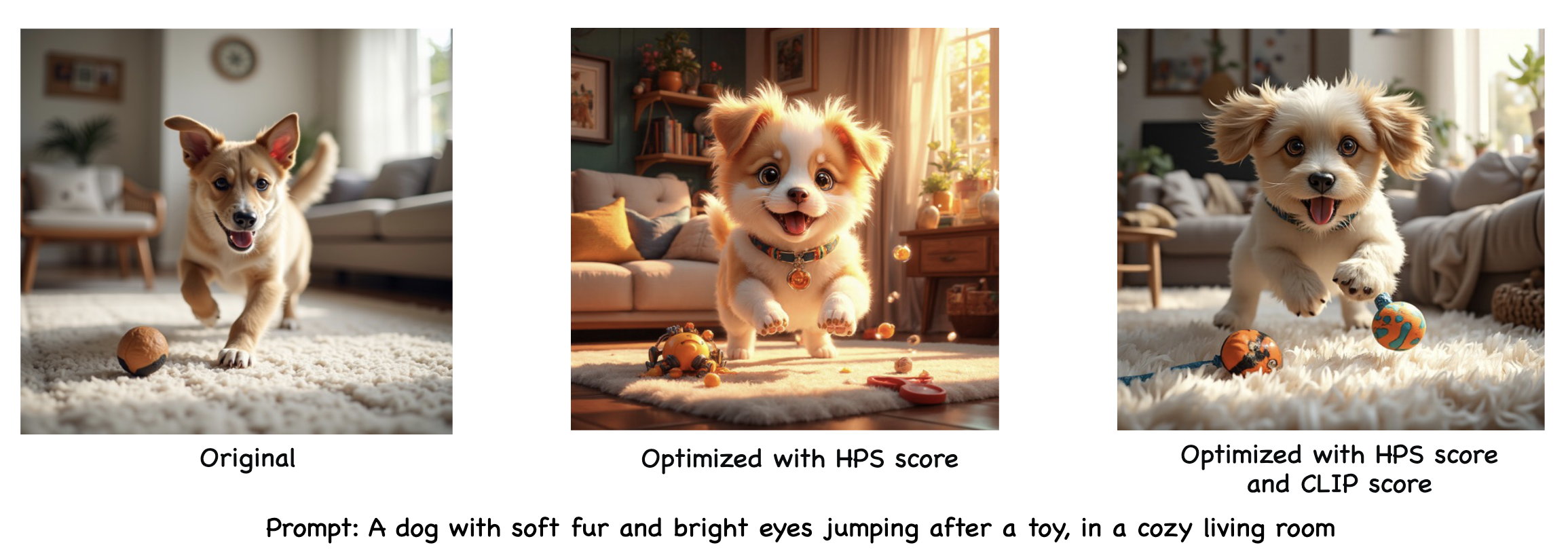
Images from DanceGRPO: Unleashing GRPO on Visual Generation (Zeyue Xue et al., 2025). Cropped; captions reformatted.
I hope this short blog was somewhat informative and interesting to read. Shoot me a message if you want to talk more about these topics.